
Understanding Predictive Performance Beyond Linear Models
Bias–variance behavior of parametric and local smoothing regression techniques in simulated settings
Introduction
The foundation of data mining is selecting appropriate models and understanding their predictive performance. I’ve explored linear regression and its variants—first for classification, then for continuous prediction—focusing on how parametric models make assumptions about data structure to minimize prediction error. Beyond parametric models are non parametric regression and local smoothing techniques, as an extension of statistical properties and computational behavior models. I compare a variety of non parametric models, KNN Regression, Smoothing Splines, Random Forest, and Boosting, in a manner of simulations. In contrast to parametric models using a fixed formula to base predictions from, these techniques can be generalized as partitioning data into segments (the different approaches are discussed in the report), with minimum to no assumption for a fixed formula. Empirical bias, variance, and mean squared error (MSE) are the measurements I compare to distinguish the performance of model practicality, using the Mexican hat function as the true function. Moreover, the experiment compares the performance of these models based on equidistant and non equidistant points in the interval -2pi and pi, which analyzes how the models perform in different scenarios of data sparsity (how data is spaced out).
1 Data Sources
I am using randomized data sets that have the underlying famous Mexican hat function f(x) = (1-x^2)exp(-0.5x^2) with x values within the range -2pi and pi:
- 101 Equidistant x points
- 101 non equidistant x points. The non equidistant points are intentionally computed with 70% of x points randomly generated near the value 0, which is the center of the domain. The remaining x points are generated across the full domain.
The data sets are randomly generated as the true Mexican Hat function plus generated error, making it the training data used to fit KNN Regression, Spline Smoothing, Random Forest, and Boosting. The testing data is the true Mexican hat function (Figure 1), used to assess model performance.
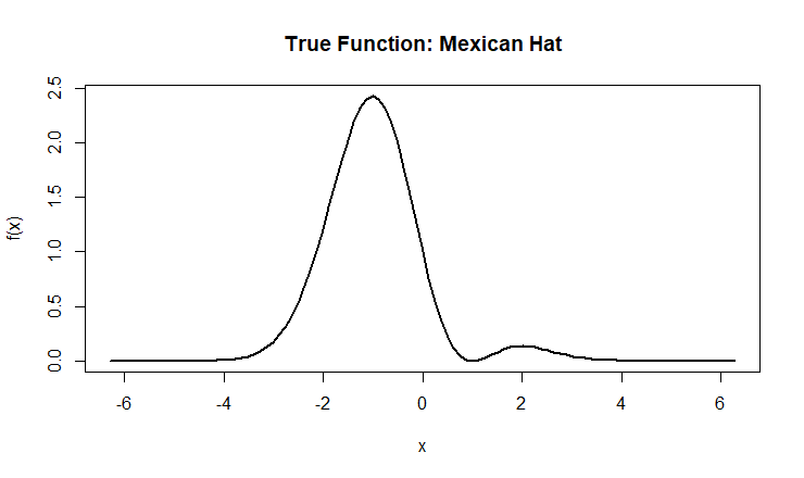
Figure 1: The Mexican function “is known to pose a variety of estimation challenges”. If a simpler function is used, it is likely that all models would perform similarity, making it hard to note the bias and variance trade offs among the models.
2 Methodology
There are two parts to this experiment, comparing KNN Regression, Smoothing Splines, Random Forest, and Boosting with the first part using equidistant x points and the second part using non equidistant x points. For each part, the Monte Carlo algorithm is used to generate 1000 observations with added noise (along the underlying function) and fitting the three non parametric models.
Conducting the experiment with a true function is a matter of theory. Typically, calculating variance and bias is numerically impossible in cases where we don’t have the true function. Because the experiment is conducted as a simulation, where randomized data sets and the true function are computed, the variance-bis trade off can be mathematically computed. MSE^2 = Bias^2 + Variance + Sigma^2 is the formula derived to compute measurements of bias, variance, and MSE.
Before generating data and fitting models in the experiment, it is necessary to tune parameters for the non-parametric models: KNN Regression, Random Forest, and Boosting. In parametric models, tuning pertains to the coefficients of a fixed linear formula. In the case of non parametric models, however, tuning prevails intensity in procedure, which leads to different interpretations for different factors between models.
The behavior of each model, tuning parameter model variables, and the effect to “intensity in procedure” is discussed below:
2.1 KNN Regression
The KNN Regression model relies on a select number (K) of data points dependent on the value of the predictor variable, known as K-Nearest Neighbors. The predicted value is the average of K closest data points closest to the value.
Tuning K in KNN Regression compares the prediction error of the model across different Ks, to select the optimal number of neighbors (K) in the K-Nearest Neighbors algorithm. The greater K is, the more prone the model is to high bias due to the nature of smoothing.
Cross validation (see appendix A) is used to select the optimal K neighbors.
2.2 Smoothing Splines
The Spline Smoothing model fits a global function, but adds a penalty that discourages the roughness of curvature. The goal is to balance how well the function fits the data versus how smooth it remains. Instead of averaging local neighbors like KNN Regression, smoothing splines use basis functions to represent the entire curve across the domain, making it more stable and smooth, especially in sparse regions.
Tuning is performed using the smoothing parameter λ, which controls the trade-off between fit and smoothness. A small λ allows the spline to closely follow the data (low bias, high variance), while a large λ produces a smoother, more generalized function (higher bias, lower variance).
Cross-validation is used to select the optimal λ.
2.3 Random Forest
Random forest is an ensemble (see appendix A) method that builds multiple decision trees and combines their predictions to improve accuracy and reduce overfitting. Each tree is trained on a bootstrap sample (see appendix A) of the data, and at each split, only a random subset of predictors is considered - which decorrelates the trees and improves performance. The final prediction is the average of all trees.
Tuning in Random Forest involves selecting parameters such as:
- Number of trees (ntrees): more trees stabilize predictions
- Number of features considered at each split (mtry = 1 for this experiment): affects variability and tree diversity
Cross-validation or OOB (see appendix A) error is used to evaluate performance across tuning values to select the optimal combination of tuning parameters.
2.4 Boosting
Boosting (see appendix A) is another ensemble method that builds trees sequentially, where each new tree is trained to correct the errors of previous trees. Instead of voting like Random Forest, boosting adds weak learners together to form a strong final model.
Tuning in Boosting involves:
- Number of trees (M): too many trees may overfit
- Learning rate (λ): smaller values improve stability but require more trees.
- Tree depth: Shallower trees reduce variance and improve generalization.
Cross validation is used to select the optimal λ.
3 Results
For reference, I am including the results of the Empirical bias, variance, and mean squared error (MSE) for the predictive performance of the models to the true mexican hat function (see appendix A).
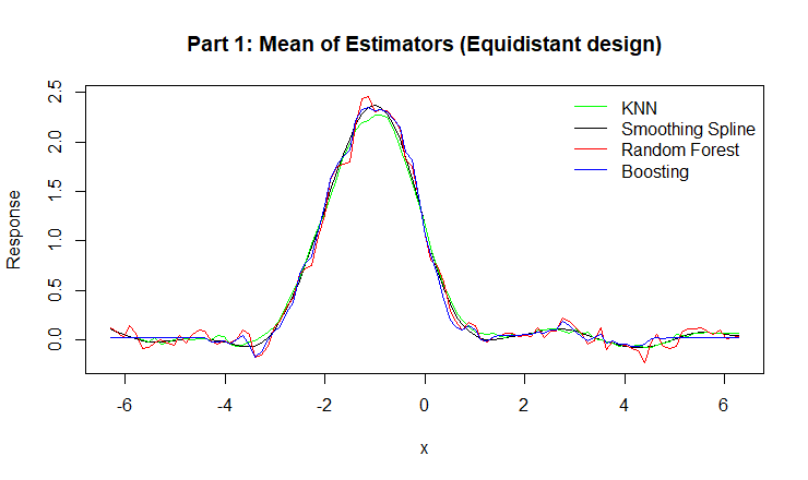
Figure 2: Mean of Estimators for KNN, Smoothing Spline, Random Forest, and Boosting.
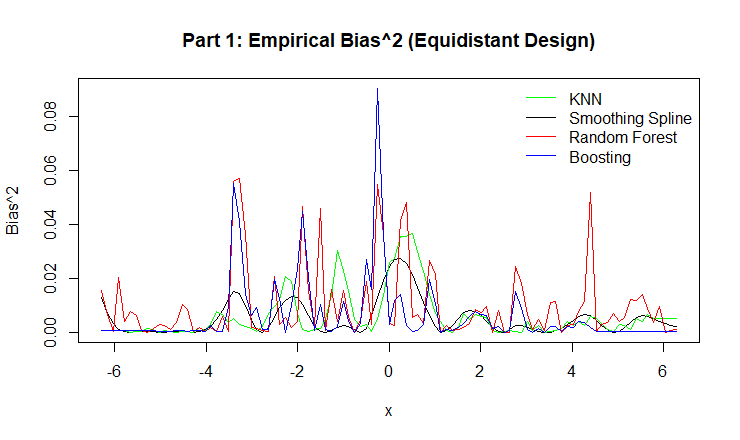
Figure 3: Empirical Bias for KNN, Smoothing Spline, Random Forest, and Boosting.
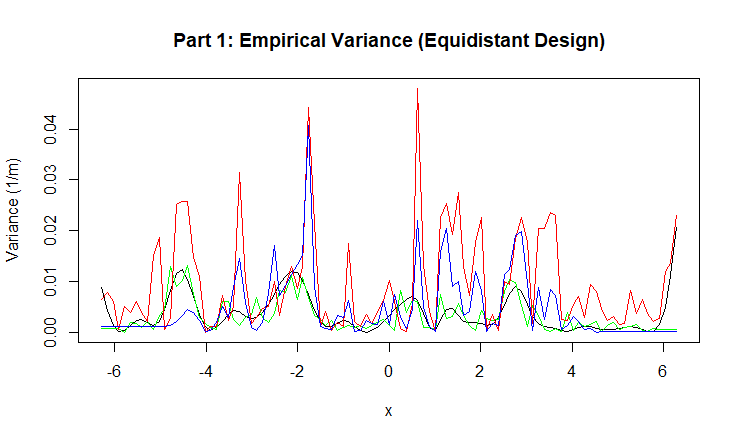
Figure 4: Empirical Variance for KNN, Smoothing Spline, Random Forest, and Boosting.
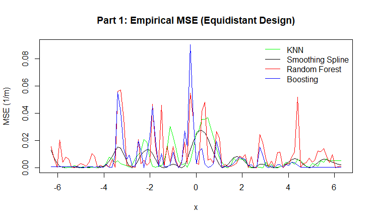
Figure 5: Empirical MSE for KNN, Smoothing Spline, Random Forest, and Boosting.
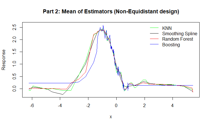
Figure 6: Mean of Estimators for for KNN, Smoothing Spline, Random Forest, and Boosting.
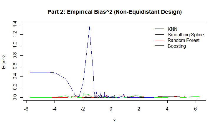
Figure 7: Empirical Bias for KNN, Smoothing Spline, Random Forest, and Boosting.
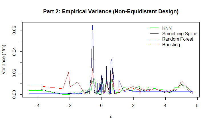
Figure 8: Empirical Variance for for KNN, Smoothing Spline, Random Forest, and Boosting.
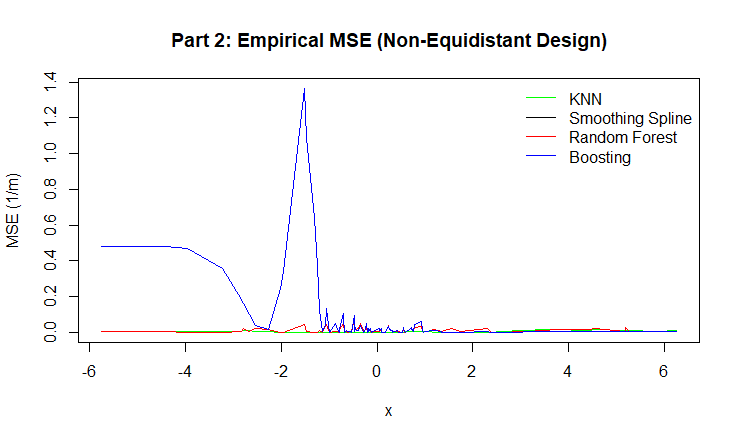
Figure 9: Empirical MSE for KNN, Smoothing Spline, Random Forest, and Boosting.
Findings/Conclusion
This experiment compared the performance of four non-parametric regression models — KNN Regression, Smoothing Splines, Random Forest, and Boosting — under both equidistant and non-equidistant designs. By simulating data from a known true function, we were able to evaluate and visualize empirical bias, variance, and mean squared error (MSE), which are normally impossible to compute when the true function is unknown in real-world data.
Across both parts, all models were able to capture the overall structure of the Mexican hat function. However, their performance differed in terms of the bias–variance trade-off.
Smoothing Splines consistently displayed smooth, low-bias curves and performed especially well in regions with sparse data, showing stability due to its global basis formulation.
KNN Regression produced locally flexible estimates, but as expected, was sensitive to data density. Its performance degraded slightly in non-equidistant regions where fewer neighbors were available.
Random Forest showed strong performance across both designs, with relatively low variance and bias. This is due to averaging across many de-correlated trees, which stabilizes predictions.
Boosting achieved high accuracy in dense regions but showed noticeable spikes in bias and MSE in sparse areas, especially in the non-equidistant design. This suggests that sequential learning can overcorrect noise when data is unevenly distributed.
In terms of overall predictive accuracy, Random Forest and Smoothing Splines offered the most consistent balance between bias and variance, while Boosting demonstrated high flexibility but was more sensitive to tuning and instability in data-sparse regions. KNN Regression remained intuitive and competitive but was dependent on local data availability and the choice of K.
This simulation confirms the theoretical relationship MSE = Bias^2 + Variance + Sigma^2 and shows how model flexibility, smoothing, and tuning directly influence each component of error. Overall, this experiment highlights that no model universally dominates; rather, model selection should depend on data structure, smoothness of the underlying function, and the trade-off between interpretability and predictive stability.
Appendix: Glossary of Terms
Bias: Measures how far the average prediction of the model is from the true underlying function.
Bootstrap sample: A random select of observations from the original dataset with replacement; repeated B times to generate B datasets.
Cross Validation: When the model is trained using different values of the tuning parameter and an average validation error is computed across all folds.
Ensemble: An approach that combines many simple models to form one final model that may potentially be more powerful.
MSE: The average of the squared differences between the model’s predictions and the true function values. It combines both bias and variance, MSE = Bias^2 + Variance
Variance: Measures how much the model’s predictions vary across different datasets. It is the average of the squared deviations of predictions from their mean prediction.